Discharge Tools¶

Catchment hydrology¶

Common tools for diagnosic tools frequently used in catchment hydrology.

flow_duration_curve¶

hydrobox.discharge.flow_duration_curve(x, log=True, plot=True, non_exceeding=True, ax=None, **kwargs)[source]¶

Calculate a flow duration curve

Calculate flow duration curve from the discharge measurements. The function can either return a matplotlib plot or return the ordered ( non)-exceeding probabilities of the observations. These values can then be used in any external plotting environment.

In case x.ndim > 1, the function will be called iteratively along axis 0.

Parameters:

x : numpy.ndarray, pandas.Series: Series of prefereably discharge measurements
log : bool, default=True: if True plot on loglog axis, ignored when plot is False
plot : bool, default=True: if False plotting will be suppressed and the resulting array will be returned
non_exceeding : bool, default=True: if True use non-exceeding probabilities
ax : matplotlib.AxesSubplot, default=None: if not None, will plot into that AxesSubplot instance
kwargs : kwargs,: will be passed to the matplotlib.pyplot.plot function

Returns:

matplotlib.AxesSubplot :: if plot was True
numpy.ndarray :: if plot was `False

Notes

The probabilities are calculated using the Weibull empirical probability. Following [1], this probability can be calculated as:

$p =m/(n + 1)$

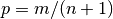
where m is the rank of an observation in the ordered time series and n are the total observations. The increasion by one will prevent 0% and 100% probabilities.

References

[1]	Sloto, R. a., & Crouse, M. Y. (1996). Hysep: a computer program for streamflow hydrograph separation and analysis. U.S. Geological Survey Water-Resources Investigations Report, 96(4040), 54.

regime¶

hydrobox.discharge.regime(x, percentiles=None, normalize=False, agg='nanmedian', plot=True, ax=None, **kwargs)[source]¶

Calculate hydrological regime

Calculate a hydrological regime from discharge measurements. A regime is a annual overview, where all observations are aggregated across the month. Therefore it does only make sense to calculate a regime over more than one year with a temporal resolution higher than monthly.

The regime can either be plotted or the calculated monthly aggreates can be returned (along with the quantiles, if any were calculated).

Parameters:

x : pandas.Series: The Series has to be indexed by a pandas.DatetimeIndex and hold the preferably discharge measurements. However, the methods does also work for other observables, if agg is adjusted.
percentiles : int, list, numpy.ndarray, default=None: percentiles can be used to calculate percentiles along with the main aggregate. The percentiles can either be set by an integer or a list. If an integer is passed, that many percentiles will be evenly spreaded between the 0th and 100th percentiles. A list can set the desired percentiles directly.
normalize : bool, default=False: If True, the regime will be normalized by the aggregate over all months. Then the numbers do not give the discharge itself, but the ratio of the monthly discharge to the overall discharge.
agg : string, default=’nanmedian’: Define the function used for aggregation. Usually this will be ‘mean’ or ‘median’. If there might be NaN values in the observations, the ‘nan’ prefixed functions can be used. In general, any aggregating function, which can be imported from numpy can be used.
plot : bool, default=True: if False plotting will be suppressed and the resulting pandas.DataFrame will be returned. In case quantiles was None, only the regime values will be returned as numpy.ndarray
ax : matplotlib.AxesSubplot, default=None: if not None, will plot into that AxesSubplot instance
cmap : string, optional: Specify a colormap for generating the Percentile areas is a smooth color gradient. This has to be a valid colormap reference, see https://matplotlib.org/examples/color/colormaps_reference.html. Defaults to 'Blue'.
color : string, optional: Define the color of the main aggregate. If None, the first color of the specified cmap will be used.
lw : int, optinal: linewidth parameter in pixel. Defaults to 3.
linestyle : string, optional: Any valid matplotlib linestyle definition is accepted.

':' - dotted

'-.' - dash-dotted

'--' - dashed

'-' - solid

Returns:

matplotlib.AxesSubplot :: if plot was True
pandas.DataFrame :: if plot was False and quantiles are not None
numpy.ndarray :: if plot was False and quantiles is None

Notes

In case the color argument is not passed it will default to the first color in the the specified colormap (cmap). You might want to overwrite this in case no percentiles are produced, as many colormaps range from light to dark colors and the first color might just default to while.

Discharge coefficients¶

Common indices frequently used to describe discharge measurements in a single coefficient.

Richards-Baker Flashiness Index¶

hydrobox.discharge.indices.richards_baker(x)[source]¶

Richards-Baker Flashiness Index

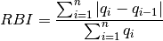
Calculates the Richards-Baker Flashiness index (RB Index), which is a extension of the Richards Pathlengh index. In contrast to the Pathlength of a signal, the R-B Index is relative to the total discharge and independend of the chosen unit.

Parameters:	x : numpy.ndarray, pd.Series The discharge input values.
Returns:	numpy.ndarray

Notes

The Richards-Baker Flashiness Index [2] is defined as:

${RBI} = \frac{\sum_{i=1}^{n}|q_i - q_{i-1}|}{\sum_{i=1}^{n} q_i}$

References

[2]	Baker D.B., P. Richards, T.T. Loftus, J.W. Kramer. A new flashiness index: characteristics and applications to midwestern rivers and streams. JAWRA Journal of the American Water Resources Association, 40(2), 503-522, 2004.